AI Demystified: How It Works Without the Complex Math - Part 1

Prakash Arumugam

26 Sep 2025 — 9 min read

Evolution of AI

This blog post is inspired by Ronald T. Kneusel's excellent book How AI Works: From Sorcery to Science.

Like many of you, I use AI tools daily in my work—from ChatGPT/Claude for brainstorming to voice assistants for quick answers. But for the longest time, I treated these systems as complete black boxes. I learned how to use them effectively, but I remained curious about the bigger questions: How did we actually get here? What's really happening under the hood that makes these tools so powerful?

If you've ever wondered the same thing—if you want to peek behind the curtain without getting lost in complex mathematics or technical jargon—this post is for you. While Kneusel's book offers deep dives into comparisons between different AI models with rich examples, my goal here is simpler: to capture the core essence of AI's evolution and its internal workings without getting lost in the details.

Think of this as the story of how humanity taught machines to think—or at least, to do a pretty convincing impression of thinking. This blog post will be divided into two parts, so it can be digested easily.

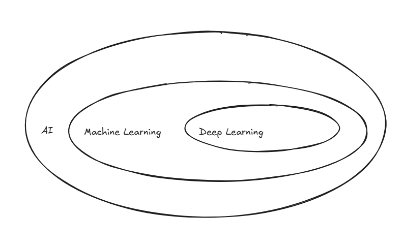
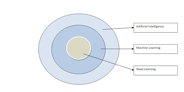
Before we dive into AI's evolution, let's clear up some terminologies AI, Machine Learning, Deep Learning that often gets jumbled together. Think of AI, Machine Learning, and Deep Learning as nested circles: AI is the biggest circle (the broad goal of creating intelligent machines), Machine Learning sits inside it as a specific approach, and Deep Learning sits inside Machine Learning as an even more specialized technique.

Machine Learning

Since machine learning has become the dominant path to AI today, let's understand how it works.

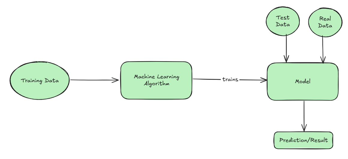
At its core, machine learning works like this: imagine you have a model (model is an abstract notion of something that accepts inputs and generates outputs, where inputs and outputs are related in some meaningful way.) —think of it as a very sophisticated pattern-recognition system. You feed it input data, it produces an output, and then you check how accurate that output is. Based on the results, the system automatically adjusts its internal parameters to get better at the task.

Here's the crucial part: the dataset is everything. The more diverse and comprehensive your training data, the better your model performs. It's like teaching someone to recognize dogs—if you only show them photos of Golden Retrievers, they'll struggle to identify a Chihuahua. Biased or incomplete datasets create biased or limited models.

To measure accuracy, data scientists use tools like confusion matrices—essentially scorecards that show where the model gets things right or wrong. But here's a key limitation: models can only make good predictions about situations similar to what they've seen before (interpolation). When they encounter completely new scenarios (extrapolation), they often fail spectacularly.

Classical Machine Learning Models

Before deep learning took center stage, several foundational approaches dominated the field, lets discuss about them briefly

Decision Trees work exactly like their name suggests—they make decisions by asking a series of yes/no questions. Imagine diagnosing whether someone has a cold: "Do they have a runny nose? If yes, do they have a fever? If no, do they have a cough?" Each branch leads to a decision. Simple and interpretable, but individual trees can be quite rigid.

Random Forests solve this rigidity by creating many decision trees and letting them "vote" on the answer. It's like asking 100 doctors for their opinion and going with the majority—more robust and accurate than relying on just one perspective.

Support Vector Machines (SVMs) take a different approach entirely. They try to find the best "boundary line" that separates different categories in your data. Think of it like drawing the optimal line to separate cats from dogs in a photo dataset—SVMs find the line that gives the maximum "breathing room" between categories.

These classical approaches worked well for many tasks and are still used today. However, they each have limitations that become apparent when dealing with complex, real-world data like images, speech, or natural language. This is where deep learning enters the story.

Deep Learning and Neural Networks - The foundation of Modern AI

AI has historically taken two main approaches

Symbolic AI - top-down, where we program explicit rules
Connectionism - bottom-up, where systems learn patterns from data

Think of symbolic AI like writing detailed instructions for every possible scenario, while connectionism is more like showing a child thousands of examples until they recognize patterns naturally. With today's processing power and vast datasets, connectionism—embodied in neural networks—has become the dominant approach.

Neural Networks

Understanding neural networks is crucial because they form the foundational architecture underlying all generative AI systems, including large language models.

Neural networks draw inspiration from how neurons in our brain process information. The basic building block of Neural network is called as "Node" (Artificial Neuron). Just like single brain neuron has limited capabilities, artificial neural networks gain power by connecting many nodes in layers - the more nodes and layers, the more complex patterns they can recognize. Below specified diagram shows a humble one node neural network on the left and two node neural network on the right side.

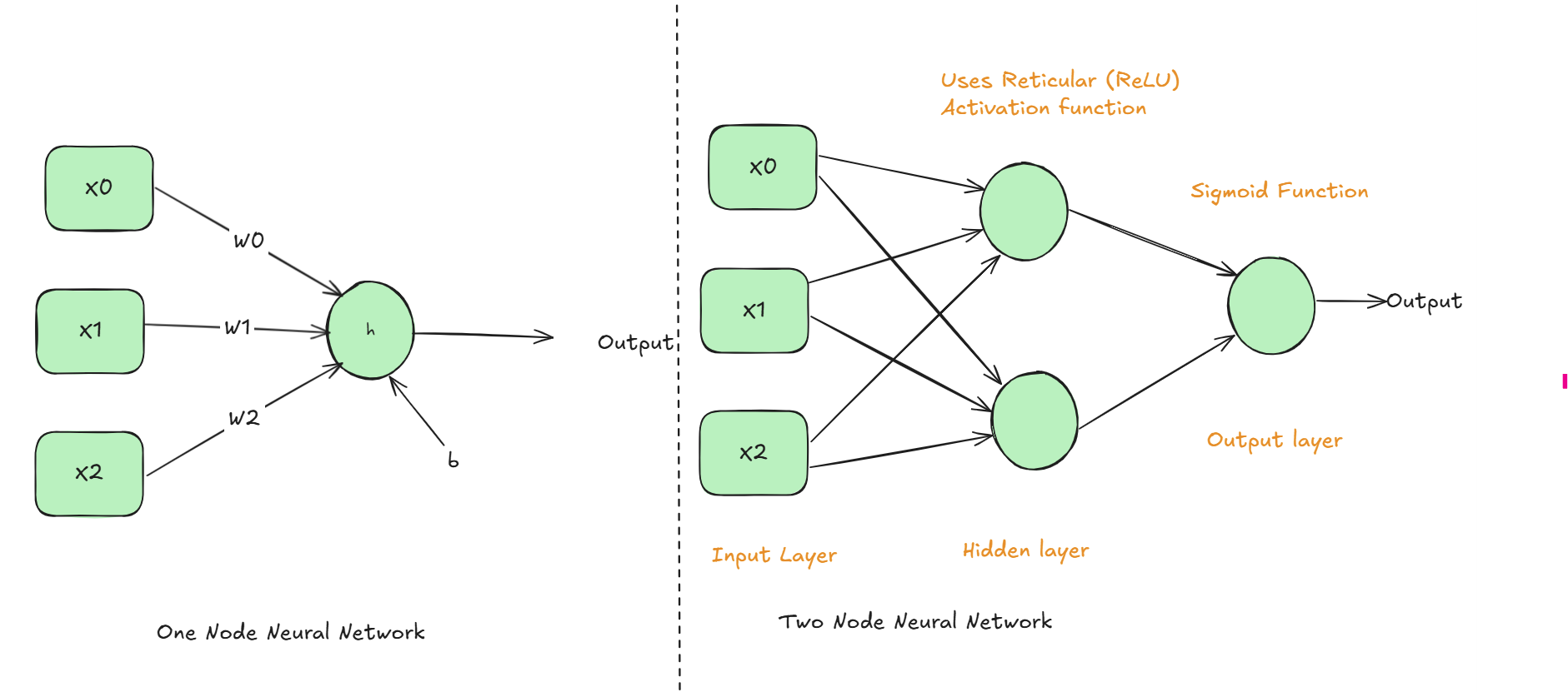
The Artificial Neuron operates like this

Multiply every input value, X0, X1 and X2 by its associated weight W0, W1 and W2.
Add all the products from the step 1 together along with the bias value "b". This produces a single number.
Input the single number to h, the activation function, to produce the output also a single number.

That's all the Neuron does, string enough Neurons together and you have a model that learn to identify different animals, drive a car or translate one language to another. Example captured at the end of this blog, will help in understanding the functionality better.

Lets briefly expand on the additional components captured in the two node neural network, before discussing about training

Hidden Layer (with ReLU)

Hidden layer acts like a filter, that decides what information is worth paying attention to. ReLU (Reticular Linear Unit) works like a bouncer at a club - it only lets positive signals through and blocks negative ones (sets them to zero).
This helps the network focus on the most relevant patterns and prevents it from getting confused by noise.

Output Layer (with Sigmoid)

This layer is like a "Confidence Translator", the Sigmoid function takes whatever number the hidden layer produces and squashes it into a probability between 0 and 1 (i.e., 0% to 100% confidence).
So instead of getting a raw number like 123.45, you get something meaningful like "0.85" i.e., 85% confident.

More the layers and nodes, neural networks can learn more complex relationships.

Important distinction with Neural networks is that they don't give you definitive answers like "this is definitely a cat." Instead, they output confidence levels: "I'm 85% confident this is a cat, 10% confident it's a dog, 5% other." During training, the network repeatedly adjusts its parameters (weights and biases) to get better at these probability judgments.

This probabilistic approach is what makes neural networks so powerful—and what laid the groundwork for today's large language models.

Training

The general training algorithm is

Preprocessing: Clean and format your data (normalize values, handle missing data etc.,)
Initialize: Start with random weights and bias throughout the network.
Forward Pass: Feed training data through the network to get predictions.
Calculate Error: Compare predictions to actual answers.
Backward Pass: Calculate how much each weight/bias contributed to the error.
Update Weights and Biases
Repeat: Go to step 3, continue this cycle thousands of times until error is minimized.

Selecting weights and bias selection is crucial and neural network uses two key techniques, Gradient descent and Backpropagation to optimally select the weights and bias which yields better predictions i.e., low error rate.

In order to understand, Gradient descent and backpropagation, imagine you're blindfolded on a hilly landscape and need to find the lowest valley (minimum error). You have millions of weights and biases to adjust, creating a complex multi-dimensional "error landscape." The challenge: how do you systematically find the combination that gives you the lowest error?

Gradient Descent - The Navigation System Think of gradient descent like using a compass that always points toward the steepest downhill direction. At any point, it calculates the "slope" of the error surface and takes a step in the direction that reduces error most quickly.

Backpropagation - The Blame Assignment Backpropagation figures out "who's responsible for the mistake." It traces backward from the final error to determine exactly how much each weight contributed to that error, so gradient descent knows which direction to adjust each parameter.

"Gradient descent uses the gradient direction supplied by backpropagation to iteratively update the weights and biases to minimize the network's error over the training set."

For Example: Let's say your network predicts a house price as $200k, but the actual price is $250k (error = $50k).

Backpropagation traces back: "Weight A contributed +$30k to the error, Weight B contributed +$20k"
Gradient descent then adjusts: "Decrease Weight A more than Weight B to reduce the error"

Neural network training can be approached in different ways depending on how much data you process before updating weights.

Batch gradient descent processes your entire dataset before making any weight adjustments—imagine reading every single book in a library before taking any notes. This is thorough but slow.
At the other extreme, you could update weights after every single example, but this approach is rarely used because it's too erratic and inefficient.
The practical standard is stochastic gradient descent (SGD), which despite its name, typically processes small chunks of data called mini-batches before updating weights—think of it as taking notes after reading a few pages rather than after each sentence or after the entire library.

An epoch represents one complete journey through your entire training dataset. So if you have 10,000 training examples and use mini-batches of 100, you'll need 100 mini-batch updates to complete one epoch. This mini-batch approach (commonly called SGD) has become the gold standard because it's computationally efficient, provides stable learning by smoothing out noise from individual examples, and makes practical use of modern hardware capabilities.

To put things in scale, GPT-3.5 (which powered early versions of ChatGPT) contained 175 billion parameters.

Below specified example ties together all the Neural Network concepts, which we discussed above

House Price Prediction Neural Network

Architecture

INPUT LAYER          HIDDEN LAYER              OUTPUT LAYER
(Normalized)        (ReLU activation)        (Linear activation)

Square feet (0.67) ─────┐
                        ├─── [Node 1] ─────────┐
Bedrooms (0.60) ────────┤    w=[0.5,0.3,0.2]   ├─── [Price Node] ─── $300,560
                        │    b=0.10            │    w=[0.8,0.6]    (denormalized)
Location (0.80) ────────┤                      │    b=0.20
                        └─── [Node 2] ─────────┘
                             w=[0.4,0.7,0.5]
                             b=0.05

Step-by-Step Process

Input: House with 2000 sq ft, 3 bedrooms, location score 8

Normalized inputs: [0.67, 0.60, 0.80] (divided by maximum values: sq ft/3000, bedrooms/5, location/10)
Note: During training, house prices were normalized by dividing by $200,000 (the maximum price in training dataset)

Hidden Layer Calculations

Node 1: (0.67×0.5) + (0.60×0.3) + (0.80×0.2) + 0.10 = 0.335 + 0.180 + 0.160 + 0.10 = 0.775 → ReLU → 0.775

Node 2: (0.67×0.4) + (0.60×0.7) + (0.80×0.5) + 0.05 = 0.268 + 0.420 + 0.400 + 0.05 = 1.138 → ReLU → 1.138

Output Layer Calculation

Output: (0.775×0.8) + (1.138×0.6) + 0.20 = 0.6200 + 0.6828 + 0.20 = 1.5028

Denormalize to actual price:

Predicted price = 1.5028 × $200,000 = $300,560

Training Example

Error calculation:

If actual price = $250,000
Absolute error = $300,560 − $250,000 = $50,560 (prediction too high)

Learning process:

Backpropagation: Traces which weights caused overestimation
Weight adjustment: Reduces weights that led to high prediction
Repeat: Process many houses to learn accurate pricing patterns

Early neural networks faced critical limitations that prevented mainstream adoption. The "vanishing gradient problem" made deep networks impossible to train effectively—learning signals became too weak to reach early layers. Limited computing power and insufficient data (pre-internet era) meant networks were either too slow to train or couldn't learn complex patterns without overfitting. These shallow networks could only handle simple tasks, leading to the "AI winter" of reduced funding and interest.

The breakthrough came when massive datasets, powerful GPUs, and architectural innovations like transformers finally provided the computational power and data scale needed to unlock neural networks' true potential.

In part-2, We will build on top of this foundation to learn about Generative AI, which uses much larger and more sophisticated versions of these same neural network principles.

References